The development of new molecules in agriculture has historically relied on classical null-hypothesis significance testing (NHST). When a new active ingredient (AI) candidate is proposed for market, the goal is typically to show that its efficacy is superior to either an untreated control or an already-marketed reference product, since demonstrating superiority is what makes it economically attractive.
Setting aside comparisons against an untreated control, this paradigm faces a critical bottleneck in agricultural product development: existing reference products are often already highly efficacious, which makes superiority difficult, or sometimes impractical, to establish under the NHST framework. Yet decisions still need to be made, with whatever data are available, at every stage of a molecule’s life cycle.
Bayesian decision frameworks remain far less common in agriculture than in clinical trials. I’d venture that one reason is the absence of the kind of standardized guidelines the pharmaceutical industry has long relied on for data collection and analysis; in their absence, each agricultural company is left to define its own good practices.
When “Significant” Isn’t the Right Question
Agricultural trials are inherently noisy, and biological products add another layer of noise on top, since their mode of action is shaped by more variables than a purely chemical molecule’s would be. Under these conditions, the frequentist superiority test (p < 0.05) forces a binary decision that fits poorly with a practical reality where small improvements over an already-strong reference are genuinely valuable, yet rarely reach statistical significance at a realistic, affordable sample size.
Let’s work through a fictional scenario. Imagine you’re the statistician on a research team tasked with deciding whether any of several candidate AIs is worth advancing further down the pipeline toward market.
Suppose a sprayable product already on the market improves corn yield (or any crop, for that matter), and your company has three candidates that showed promise in greenhouse trials. The proof-of-concept bar for any of them to advance is a yield improvement of at least 3% over the reference.
Ideally, if the performance of the candidates is robust enough, the greenhouse findings would easily be replicated in the field. However, that rarely happens, unless you win the lottery of finding a holy grail candidate among a pool of thousands.
Based on your experience handling low, noisy signals from earlier development ingredients with no historical data to inform a power analysis, you propose, as part of the Statistical Analysis Plan, a sample size of 5 trials across five locations, with 3 replicates per treatment. However, after several stakeholder meetings, logistic and financial constraints (scarce AI quantities, high equipment costs) force the affordable sample size down to 3 trials, with 3 replicates per treatment.
Will this be enough to get a clear yes/no answer? Let’s create a realistic scenario to find out.
Creating our Realistic Fake Data
Click here to skip the technical details of the simulation.
The most commonly used design of experiments in agriculture is the Randomized Complete Block Design (RCBD). When applied to a single trial, its analysis is referred to as Single Trial Statistics. This analysis is useful for registration purposes, as its main goal is to statistically back up the candidate’s efficacy over an untreated control. However, all candidates are chosen at the bottom of the pipeline because their advantages over an untreated control have already been demonstrated in preliminary assays (e.g., laboratory studies, greenhouse trials). Hence, knowing that they are better than the untreated control is not particularly useful for decisions where the actual question is whether the candidate shows potential to compete with whatever product is already on the market.
In that sense, an RCBD applied over multiple trials becomes more informative and powerful, as it models more sources of variation that could affect the performance of the candidates. In this case, its analysis takes the name of Trial Series Statistics, and it constitutes the baseline for the rest of this post.
A typical Trial Series Analysis can be performed using the following equation:
\(u_j \sim N\left(0,\sigma^2_{trial}\right)\) : random trial effect
\(b_{k(j)} \sim N\left(0,\sigma^2_{block}\right)\): random block nested in trial
\(g_{ij} \sim N\left(0,\sigma^2_{treatment:trial}\right)\): random treatment:trial interaction
\(\epsilon_{ijk}\): residual error
Our aim in this section is to simulate data that resembles real data as closely as possible. For this, we will assume:
We’re not concerned with an untreated control for this exercise.
The reference product (call it “Treatment 1”) has a true mean yield of 100 bushels per acre (Bushel/acre). Treatments 2 through 4, our three candidates, differ from it by 0%, 3%, and 5% respectively. These differences represent the effect sizes of interest: true mean yields of 100, 103, and 105 Bushel/acre for Treatments 2, 3, and 4.
Since we’ll analyze the data as a trial series analysis, we need to specify the variance components of the model up front (the random intercepts depicted above).
This last part is crucial: the variance components determine how easy it will be to find statistical significance. The smaller they are, the easier it is; the larger they are, the closer the results get to pure random noise.
So, first we need to find a reasonable set of values for them. From my personal experience (in the units used here), typical trial variance ranges from 6 to 12, trial:block variance from 2 to 3, treatment:trial interaction variance from 1 to 3, and residual variance from 3 to 6.
Keeping in mind that early-phase development trials usually show very poor power, we will choose a set of variance components likely to produce power values below 10% for the treatment whose true mean we know outperforms the reference by 5 bushels per acre.
If you are interested in reviewing the simulation routine, you can click on the Show the code button below.
Show the code
library(lme4)library(emmeans)library(dplyr)library(tibble)# 1. We create a function to simulate 200 data sets with provided variance components and compute their statistical power.simulate_power <-function(trial_sd, block_sd, gxe_sd, residual_sd,n_trials =3,n_blocks =3,n_reps =200){ pvals <-numeric(n_reps)for(i inseq_len(n_reps)){# Simulate data design_data <-expand.grid(Trial=factor(1:n_trials),Block=factor(1:n_blocks),Treatment=factor(c("Treatment_1","Treatment_2","Treatment_3","Treatment_4"),levels=c("Treatment_1","Treatment_2","Treatment_3","Treatment_4")) ) design_data$Trial_Block <-interaction(design_data$Trial, design_data$Block) design_data$Treatment_Trial <-interaction(design_data$Treatment, design_data$Trial) trt_effects <-c(0,0,3,5) trial_eff <-rnorm(nlevels(design_data$Trial),0, trial_sd) block_eff <-rnorm(nlevels(design_data$Trial_Block),0, block_sd) gxe_eff <-rnorm(nlevels(design_data$Treatment_Trial),0, gxe_sd) design_data$y <-100+ trt_effects[design_data$Treatment] + trial_eff[design_data$Trial] + block_eff[design_data$Trial_Block] + gxe_eff[design_data$Treatment_Trial] +rnorm(nrow(design_data),0,residual_sd)# Fit the model mod <-suppressMessages(lmer( y ~ Treatment + (1|Trial)+ (1|Trial:Block)+ (1|Treatment:Trial),data=design_data ) ) em <-emmeans(mod,~Treatment) dunnett <-contrast(em,method="trt.vs.ctrl",ref="Treatment_1",adjust="dunnett") |>as.data.frame() pvals[i] <- dunnett$p.value[ dunnett$contrast=="Treatment_4 - Treatment_1" ] }mean(pvals<0.05)}
Once we have run the simulations, we look at the first 10 sets of variance components whose power is near 10%:
From the output above, let’s choose the values of 10, 2, 3, and 4 for the trial, trial:block, treatment:trial and residual variance components, respectively.
One more step remains. What we are trying to accomplish in this section is to create a realistic data set where NHST falls short, while still ensuring the simulated values are consistent with the true means we established. With the values chosen above, running a large enough number of simulated data sets would, on average, converge to the true values. However, we specifically need to confirm that for just 3 trials, the simulated averages remain close to the true ones.
To do this, we will simulate several data sets with these variance components and select the random seed that produces a reasonable root mean square error between the simulated values and their true means, together with a non-significant p-value for Treatment 4 and a reasonable coefficient of variation.
Finally, from the results above, we pick the data set simulated with seed 76 for the rest of the example, since it satisfies all the criteria we set out.
Analyzing the Trial Series Analysis
Returning to our fictional scenario, the trials have already been successfully completed, and the data look like this:
Show the code
# 0. Load all required packageslibrary(ggplot2)library(dplyr)library(lmerTest)library(emmeans)library(brms)library(kableExtra)# 1. We set the general parameters for the simulationset.seed(76)n_trials <-3n_blocks <-3n_treatments <-4# Overall meanmu <-100# Fixed treatment effectstrt_effects <-c(Treatment_1 =0,Treatment_2 =0,Treatment_3 =3,Treatment_4 =5)# Standard deviations of random effectstrial_sd <-10block_sd <-2gxe_sd <-3residual_sd <-4# 2. Experimental layout design_data <-expand.grid(Trial =factor(1:n_trials),Block =factor(1:n_blocks),Treatment =factor(names(trt_effects), levels =names(trt_effects)))# Block nested within Trialdesign_data$Trial_Block <-interaction(design_data$Trial, design_data$Block,sep =":")# Treatment × Trial interactiondesign_data$Treatment_Trial <-interaction(design_data$Treatment, design_data$Trial,sep =":")# 3. Simulate random effects # Trial effectstrial_effects <-rnorm(nlevels(design_data$Trial),mean =0,sd = trial_sd)names(trial_effects) <-levels(design_data$Trial)# Trial:Block effectsblock_effects <-rnorm(nlevels(design_data$Trial_Block),mean =0,sd = block_sd)names(block_effects) <-levels(design_data$Trial_Block)# Treatment × Trial interaction effectsgxe_effects <-rnorm(nlevels(design_data$Treatment_Trial),mean =0,sd = gxe_sd)names(gxe_effects) <-levels(design_data$Treatment_Trial)# Residual errorsresidual_errors <-rnorm(nrow(design_data),mean =0,sd = residual_sd)# 4. Generate response design_data$y <- mu + trt_effects[design_data$Treatment] + trial_effects[design_data$Trial] + block_effects[design_data$Trial_Block] + gxe_effects[design_data$Treatment_Trial] + residual_errorsp1 <-ggplot(design_data,aes(Treatment, y, color = Trial)) +stat_summary(fun = mean, geom ="point", size =3) +stat_summary(aes(group = Treatment),fun = mean,geom ="crossbar",width =0.6,color ="black" ) +stat_summary(aes(group = Treatment,label =sprintf("%.2f", after_stat(y))),fun = mean,geom ="text",color ="black",vjust =-0.8,size =4 ) +theme_bw() +labs(y ="Observed mean of treatment per trial\n(Bushel/acre)",title ="Overall yield obtained per treatment/trial",caption ="Black segment represents the overall mean of the treatment across all trials")+theme(plot.caption =element_text(hjust =0))p1
Notice how the observed overall means show Treatments 3 and 4 pulling away from the reference by approximately 4 and 6 bushels per acre, respectively. This preliminary look leads non-statistical stakeholders on the project to grow optimistic that we might have found a suitable candidate with clear statistical significance.
As the statistician on the project, you now fit the trial series analysis model to obtain the p-values needed to decide whether any candidate meets the proof-of-concept bar.
A trial series analysis of this kind can be easily fitted with the following code:
None of the candidate treatments differ significantly from the reference. Within the classical NHST framework, this leaves us without a conclusive basis for a decision.
This scenario plays out often enough in practice that, under pressure from stakeholders, decisions frequently fall back on qualitative judgment (typically the expertise of field agronomists). There’s nothing wrong with that in itself, but it raises the question: what if we had a decision framework better suited to this kind of noisy, high-baseline-efficacy data in the first place?
Power Analysis: How Many Trials Would NHST Actually Need?
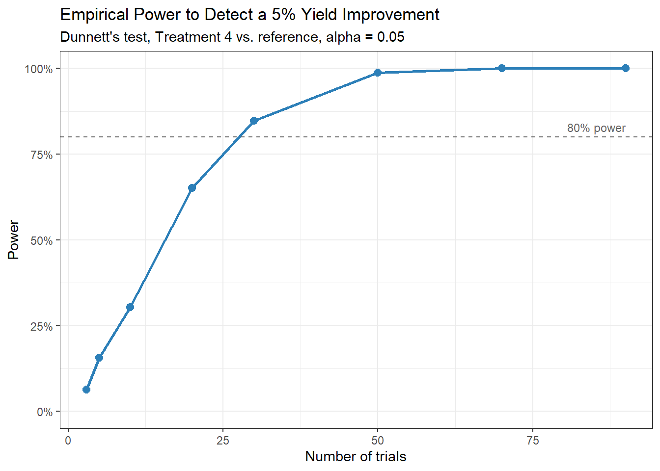
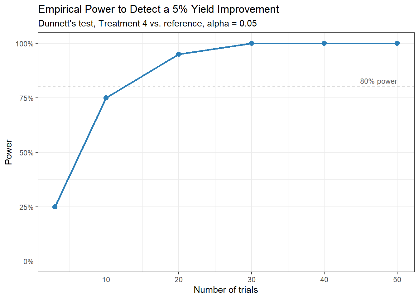
Before jumping to a Bayesian alternative, it’s worth asking a more basic question: could we simply run more trials until NHST gives us a clear answer? Let’s check empirically, using the same data-generating process as above, varying only the number of trials and focusing on the treatment whose simulated effect size we know clears the proof-of-concept bar (Treatment 4, with 5% higher yield than the reference).
Even with 20 trials, power hasn’t fully plateaued near 100%, and reaching the conventional 80% threshold requires somewhere in the range of 10-20 individual field trials (for a single candidate, against a single reference, for a single crop!). That’s not a realistic research program; it’s a different research program, one no agricultural company runs for a single proof-of-concept decision in one season.
This is the quantified version of the problem the introduction described qualitatively: NHST isn’t merely inconvenient here, it demands evidence at a scale the applied research process cannot practically supply. The question, then, isn’t “how do we get a significant p-value?” It’s “what can we responsibly conclude from the data we can actually afford to collect?”
A Bayesian Alternative
Rather than forcing a yes/no answer out of the same three trials, let’s ask a different set of questions of the exact same data: how much more probable is it that each candidate is truly superior to the reference, and how strongly do the data actually favor that conclusion over “no real difference at all”?
We refit the same random-effects structure as the GLMM above (including trial, trial-block, and treatment-by-trial variance), but now as a Bayesian hierarchical model, with weakly informative priors on the fixed effects and variance components.
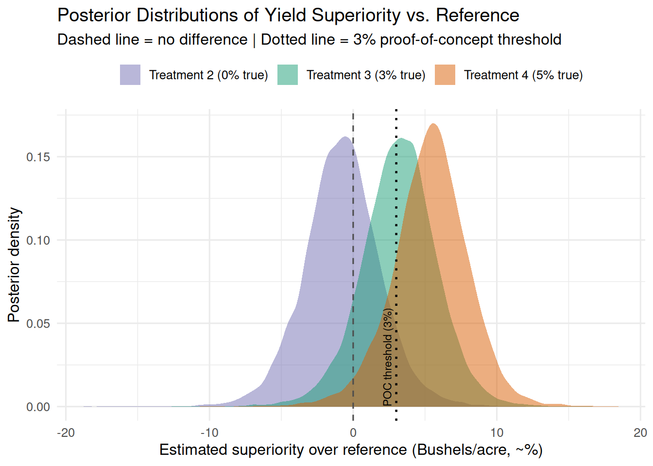
From the posterior draws, we can ask exactly the question the proof-of-concept criterion cares about, which is not “is p < 0.05,” but “how probable is a 3%-or-greater improvement, given what we observed?” and how strongly do the data themselves favor a real difference over no difference at all, independent of how we choose to threshold a probability?
For the first question, we simply look at the sampled posterior distribution and count how often each treatment outperforms the reference beyond the POC criterion. This gives us directly interpretable probabilities.
For the second question, we turn to Bayes factors (BF), which, without getting too deep into the technicalities, we can simply define as a measure of how strongly the data at hand support the aforementioned probabilities holding true.
For interpreting these, we rely on the Kass & Raftery (1995) BF scale, defined below:
BF10 range
Interpretation
1 – 3
Anecdotal — barely worth mentioning
3 – 10
Moderate evidence
10 – 30
Strong evidence
30 – 100
Very strong evidence
> 100
Decisive evidence
(Adapted from Jeffreys’ original scale, as popularized by Kass & Raftery, 1995.)
We find that Treatments 3 and 4, the candidates with true 3% and 5% advantages, show 54.1% and 83.7% posterior probabilities of clearing the POC bar outright. Treatment 2, by contrast, shows a much weaker probability (7.0%). None of this was visible from the Dunnett’s test above, not because the Bayesian model found something the frequentist one couldn’t, but because it’s answering a more useful question with the same noisy data.
Show the code
knitr::kable(bf_table, align ="lcc")
Treatment
P(delta > 3%, meets POC)
Bayes Factor (BF10)
Treatment_2
0.070
0.12
Treatment_3
0.541
1.90
Treatment_4
0.837
8.27
Notice, though, that only Treatment 4 reaches a BF in the moderate-evidence range (8.27); by the Kass & Raftery scale, Treatments 2 and 3 remain barely worth mentioning on their own. So far, this is the honest picture: three trials produce a promising signal, not a verdict. And that, in a way, is the whole point of this approach: rather than forcing a binary “not significant” answer, it preserves that signal instead of discarding it outright, leaving room for it to be weighed alongside the kind of field-agronomist expertise that, under the classical framework, is often the only decision-making resource left once the p-value comes back non-significant.
Where This Could Actually Go
A promising-but-inconclusive signal after one season isn’t a dead end under this framework the way a non-significant p-value effectively is; it’s a starting point. Each additional season of trials doesn’t have to be analyzed in isolation: the posterior from this season’s three trials can serve as the prior for next season’s, letting evidence accumulate naturally across a growing multi-season data pool, rather than resetting to zero every time. Over several seasons, that accumulated evidence could plausibly reach the same conclusiveness the earlier power analysis showed NHST would need 10-20 trials, within a single season, to achieve, except spread out affordably across time instead of demanded all at once.
This isn’t free, though, and it’s worth being upfront about the real costs of running a program like this in practice:
Compute scales with model complexity, not just data size. A single hierarchical model with three treatments and three trials fits in seconds. A multi-season model accumulating years of trial data, potentially with more candidates, more sites, and richer variance structures, can push MCMC sampling from a minutes-long job to something that needs real compute infrastructure, not something every team can spin up next to a spreadsheet.
Bayesian pipelines need engineering, not just statistics. Reproducible priors-updating-into-posteriors across seasons requires a proper data- and model-versioning pipeline; this doesn’t happen by rerunning a script by hand each year without something keeping track of what fed into what.
The organizational shift matters as much as the technical one. A probability and a Bayes factor require a different kind of conversation with stakeholders than “significant or not.” That’s a real adoption cost, independent of the math being sound.
None of that makes the case against trying; if anything, it’s the argument for starting the data pool now rather than later, since the earlier a program begins accumulating seasons under a consistent Bayesian pipeline, the sooner those computational and organizational costs turn into a genuine asset instead of a one-off analysis.